
If you have ever meddled with data in Python, you would have probably used the Pandas library which was specifically written for data manipulation and analysis, its most popular use is the manipulation of tabular data in DataFrames. The data I will be working with to demonstrate the functionality of the Pandas library is the Titanic dataset, the below figure (Fig. 1) shows the steps taken to get the CSV data from the specified URL into a DataFrame.
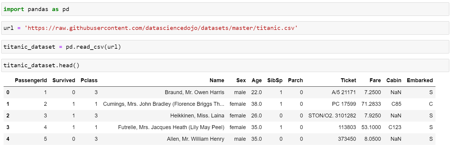
Since we now have the dataset in a DataFrame, we can perform data manipulation, before we begin; it is always good practice to create a copy of the original DataFrame in case there is a need to backtrack, for this purpose we simply assign the DataFrame to another variable.
The first useful method I will be discussing is the .info() method which returns the number of records within the DataFrame, the column names, the number of non-null values for each column as well as the data type for each column. The actual output of the method is shown in Fig. 2.
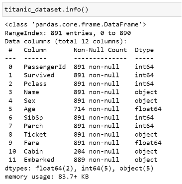
The .info() method essentially summarises the DataFrame by providing us with the key information required to gauge exactly the kind of data we are dealing with, it especially comes in handy when we first import the data to determine whether the dataset we are using could prove useful for our analysis.
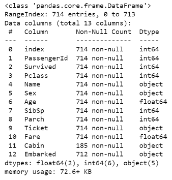
The next method I want to discuss is the .dropna() method which is used for dropping records where one of the fields for that record contains a null value; in other words its empty. Looking back at Fig. 2, we can see that the Age field contains 714 non-null values, suppose we want to perform an analysis of the dataset where the Age field is our focus, in this case, we can use a subset parameter within the .dropna() method to specify which records will be dropped based on the values within that field, hence if the field contains null value; the entire record from the DataFrame will be dropped.

In the above figure (Fig. 3) we can see that the .dropna() method in this case specifies the Age field as the subset and a parameter inplace set to true which performs the method on the current DataFrame and returns nothing. Since we have dropped some of the records within the DataFrame, resetting the index is crucial as all the records will still have their original index values even after dropping nulls, we can then drop the old index field since we have just reassigned the records to new index values. Using the .info() method again, we can see from the below figure (Fig. 4) that the new count for fields that had a greater number of non-null values than the Age field is now the same as the Age field. This method is extremely useful as it provides the means to prepare the data before it is analyzed by dropping records that contain null values.
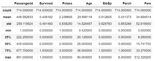
Another method that proves to be useful is the .describe() method which provides the count, mean, standard deviation, min, 25th percentile, 50th percentile, 75th percentile, and max for all numerical columns within the DataFrame to which the method is applied, in our case the resulting table of results is shown in the below figure (Fig. 5), the method serves as an analysis tool to gauge the values within the different fields.
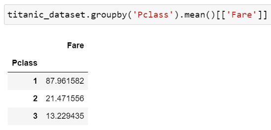
The next method in question is the .groupby() method which groups the specified column, however, we also need to specify the compute operation we want to perform on the grouped data, as can be seen in the below figure (Fig. 6), the Pclass field is grouped in this case which only contains 3 values, mean is then used as the desired compute operation to be performed and since I am only interested in the Fare field I can specify it by extracting the column from the DataFrame generated by the code below. From the results, we can see that the higher the class the higher the ticket fare, which is obvious, however, it is reassuring when the data confirms it.
The last method I want to look at is the .corr() method which returns a DataFrame containing the correlation coefficients between all the numerical columns, the result in our case is shown in the below figure (Fig. 7).
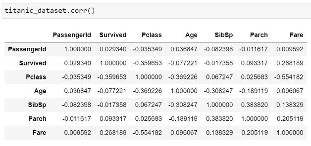
This method comes in handy when there is a need to find any relationships there may be amongst the fields, the negative sign specifies a negative correlation, and the correlation coefficient value is between 0 and 1, 1 indicating perfect correlation and 0 indicating there is no correlation. This method is extremely useful when building a regression model which is a model that describes the relationship between one or more independent variables and a target variable. In this instance, we can see that there is a fairly positive relationship between the Fare and the Survived column with a correlation coefficient of 0.268 meaning this suggests that the higher the fare amount the higher the chances of survival.
For further information on the Pandas library, please visit the official website: https://pandas.pydata.org/docs/index.html
